
Mapeo de Minerales de Alteración
Dibuje su área de licencia y reciba un mapa de alteración clasificado: argílica avanzada, fílica y propilítica, resuelto por píxel.
Mineralogía de alteración por píxel que separa asociaciones argílica avanzada, fílica y propilítica.
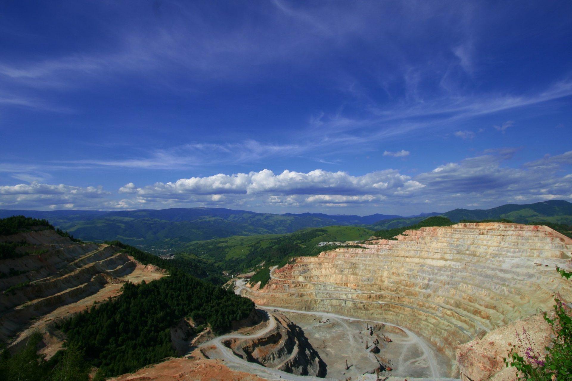
A historic mining district in Nevada. Continuum-removed alteration assemblage: advanced argillic (alunite, pyrophyllite) against phyllic (illite, muscovite).
LO QUE VE EL SENSOR
Qué busca esta capa.
La referencia de laboratorio de cada material, y qué captura de ella el espaciado de bandas del sensor. La banda sombreada marca el rango que lee el método.
QUÉ ENCUENTRA
Qué detecta.
| Material | Entorno típico | Qué puede confundirlo |
|---|---|---|
| Alunite & Pyrophyllite | High-sulfidation epithermal lithocaps and porphyry cores | Strong atmospheric water vapour at the edge of the window |
| Kaolinite & Dickite | Intermediate argillic alteration and weathering horizons | Poorly crystalline smectite clay mixtures |
| Illite & Muscovite (White Mica) | Phyllic alteration shells in porphyry Cu-Mo-Au systems | Dry canopy cellulose, which overlaps the same range |
| Chlorite & Epidote | Distal propylitic alteration haloes | Calcite and dolomite carbonate absorptions |
MÉTODO
Cómo funciona.
Entra reflectancia calibrada, y cada píxel se ajusta contra una biblioteca pública de referencia.
Surface reflectance ingest
Scenes are read at the archive's own surface reflectance level. Wherever the instrument measured nothing, that gap is declared and carried through, never interpolated across.
Continuum removal
A convex upper hull is fitted across the working range so the shape of each absorption stands apart from overall brightness.
Least-squares fitting against reference spectra
Continuum-removed features are fitted to laboratory reference spectra using non-negative least squares with wavelength shift.
Evaluability masking
Green canopy, cloud, shadow and low-illumination pixels go into a separate "not evaluated" class, hatched in the legend, transparent on the map, null in exports. Not measured is drawn differently from measured zero.
ESPECIFICACIONES
Qué obtiene, y sobre qué corre.
Condiciones que necesita
Method and checks are documented in Axine Applied Spectroscopy Paper #1 · Section 4.2.
Alcance
Reads exposed rock and soil. Vegetated and covered ground is masked out, and nothing here speaks to what lies at depth.
EJECÚTELO SOBRE SU TERRENO
Ejecute esta capa sobre su propia área.
Ordene procesamiento sobre su área de interés, o una captura programada donde el archivo no tenga nada utilizable. El acceso a las imágenes nunca se cobra: un plan compra los modelos.
ANALÍTICA COMPLEMENTARIA
Capas relacionadas.
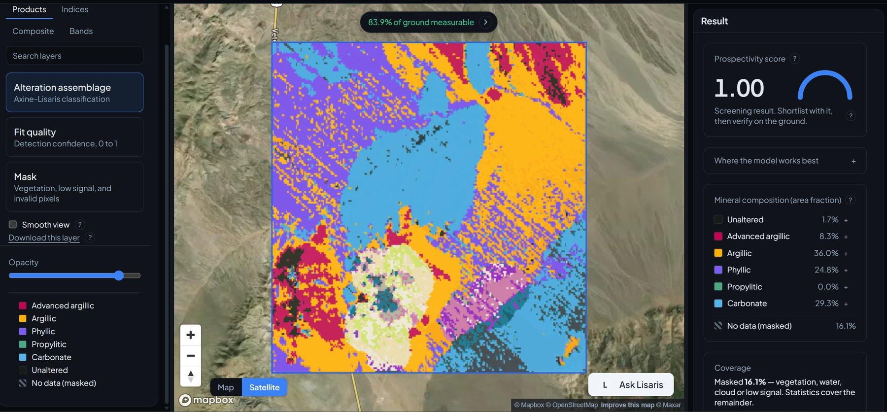
Detección de Clústeres de Alteración
Agrupamiento vectorizado que extrae los núcleos hidrotermales centrales y los nodos desde los que vale la pena trabajar hacia afuera.
Clasificación de Prospectividad Distrital
Puntuación regional de probabilidad para sistemas hidrotermales, respaldada por validación cruzada dejando una región fuera.
Vectorización de Pórfidos Cu-Au
Vectoriza hacia el centro hidrotermal siguiendo cómo cambia la composición de la mica blanca a través del distrito.